The Bitcoin quantile regression model provides a powerful and flexible approach to forecasting Bitcoin prices and understanding the factors that influence its volatile behavior across different points of its distribution. Unlike traditional linear regression, which focuses on predicting the conditional mean, quantile regression allows us to estimate the conditional quantiles (e.g., the 10th percentile, median, or 90th percentile) of the Bitcoin price distribution. This is crucial for risk management and decision-making, as it provides insights into potential downside risks and upside potential beyond average predictions.
The core idea behind quantile regression is to minimize a weighted sum of absolute errors, where the weights depend on the chosen quantile level. For example, to estimate the 0.25 quantile (the value below which 25% of the data falls), errors below the quantile are weighted by 0.25, while errors above the quantile are weighted by 0.75. This asymmetry in the weighting scheme encourages the model to fit the specified quantile more accurately than simply minimizing the overall sum of squared errors.
The advantages of using a quantile regression model for Bitcoin price analysis are numerous. First, it is robust to outliers. Bitcoin’s price history is characterized by extreme price swings, which can heavily influence the results of ordinary least squares (OLS) regression. Quantile regression, by focusing on specific quantiles and using absolute errors, is less sensitive to these outliers. Second, it does not require strong assumptions about the distribution of the error term. Unlike OLS regression, which assumes normally distributed errors, quantile regression is distribution-free, making it suitable for analyzing Bitcoin prices which often exhibit non-normal distributions. Third, quantile regression allows us to explore the heterogeneous effects of explanatory variables across the entire distribution of Bitcoin prices. For instance, the impact of trading volume on Bitcoin price may be different at the low end of the distribution (periods of market fear and potential crashes) compared to the high end (periods of exuberance and potential bubbles).
When building a Bitcoin quantile regression model, one must carefully select the appropriate explanatory variables. Common candidates include: * **Market factors:** Trading volume, volatility indices (like VIX or Bitcoin-specific volatility measures), market capitalization. * **Macroeconomic indicators:** Interest rates, inflation rates, exchange rates, and economic growth indicators. * **On-chain metrics:** Number of active addresses, transaction fees, hashrate, and coin supply. * **Sentiment analysis:** Social media sentiment, news articles sentiment related to Bitcoin. * **Lagged Bitcoin prices:** Past Bitcoin prices to capture momentum effects and potential autocorrelation.
The estimated quantile regression coefficients can then be interpreted as the marginal effect of a given explanatory variable on the specific quantile of the Bitcoin price distribution. For example, a positive coefficient for trading volume at the 0.9 quantile suggests that higher trading volume is associated with higher potential Bitcoin prices at the upper end of the distribution. By examining the quantile regression coefficients across different quantiles, we can gain a comprehensive understanding of how these factors influence Bitcoin prices under different market conditions.
In conclusion, the Bitcoin quantile regression model offers a valuable tool for risk management, trading strategies, and understanding the drivers of Bitcoin prices. Its ability to capture heterogeneous effects across the price distribution, robustness to outliers, and distribution-free nature make it a more insightful approach than traditional linear regression for analyzing this volatile and complex asset.
 640×640 total bitcoin existence reward block scientific from www.researchgate.net
  705×362 instacart delivers time quantile regression mathieu from tech.instacart.com
 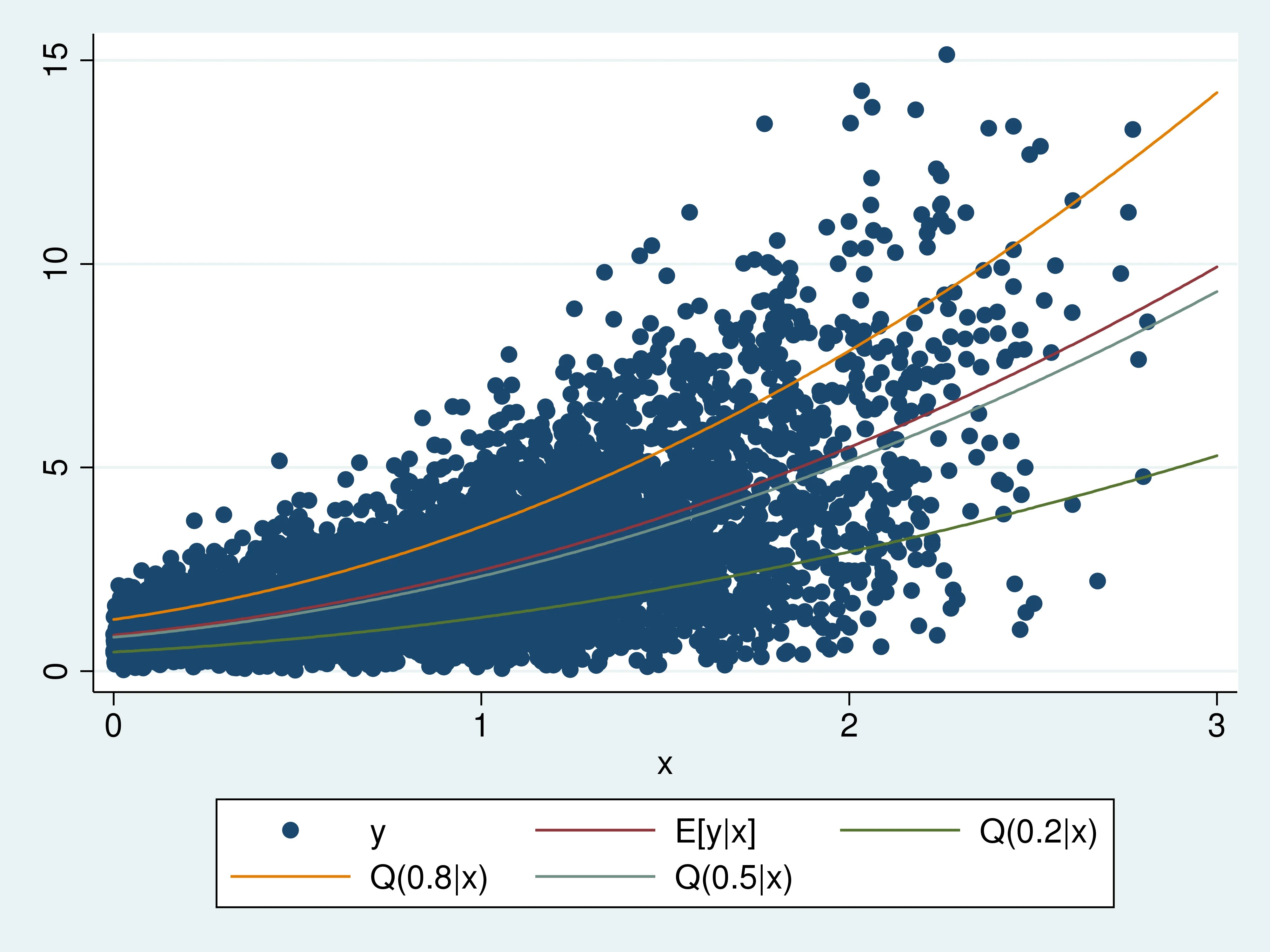 4000×3000 stata blog quantile regression covariate effects differ from blog.stata.com
  908×658 quantile regression stata advantages model from statswork.com
Leave a Reply